country happiness score by economy GDP
country happiness score by economy GDP and freedom index
Linear regression is a linear model, e.g. a model that assumes a linear relationship between the input variables (x) and the single output variable (y). More specifically, that output variable (y) can be calculated from a linear combination of the input variables (x).
On the image above there is an example of dependency between input variable x and output variable y. The red line in the above graph is referred to as the best fit straight line. Based on the given data points (training examples), we try to plot a line that models the points the best. In the real world scenario we normally have more than one input variable.
Each training example consists of features (variables) that describe this example (i.e. number of rooms, the square of the apartment etc.)
n - number of features
Rn+1 - vector of n+1 real numbers
Parameters of the hypothesis we want our algorithm to learn in order to be able to do predictions (i.e. predict the price of the apartment).
The equation that gets features and parameters as an input and predicts the value as an output (i.e. predict the price of the apartment based on its size and number of rooms).
For convenience of notation, define X0 = 1
Function that shows how accurate the predictions of the hypothesis are with current set of parameters.
xi - input (features) of ith training example
yi - output of ith training example
m - number of training examples
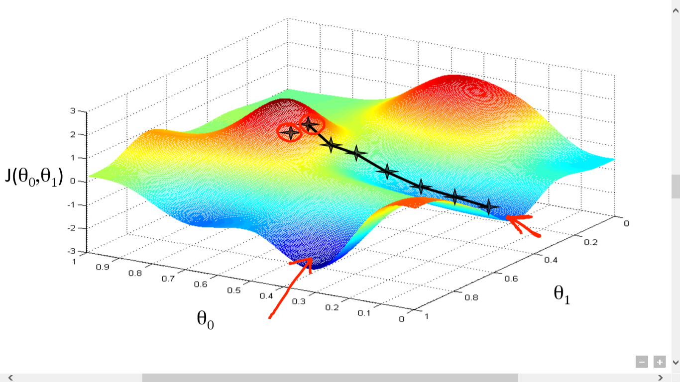
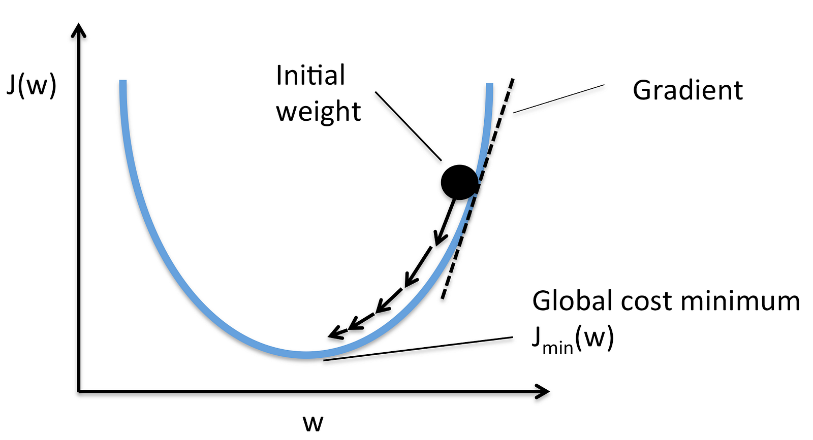
Gradient descent is an iterative optimization algorithm for finding the minimum of a cost function described above. To find a local minimum of a function using gradient descent, one takes steps proportional to the negative of the gradient (or approximate gradient) of the function at the current point.
Picture below illustrates the steps we take going down of the hill to find local minimum.
The direction of the step is defined by derivative of the cost function in current point.
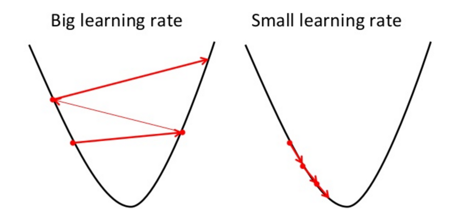
Once we decided what direction we need to go we need to decide what the size of the step we need to take.
We need to simultaneously update 


yi - output of ith training example
m - number of training examples
n - number of features
When we use term "batch" for gradient descent it means that each step of gradient descent uses all the training examples (as you might see from the formula above).
To make linear regression and gradient descent algorithm work correctly we need to make sure that features are on a similar scale.
For example "apartment size" feature (e.g. 120 m2) is much bigger than the "number of rooms" feature (e.g. 2).
In order to scale the features we need to do mean normalization


Polynomial regression is a form of regression analysis in which the relationship between the independent variable x and the dependent variable y is modelled as an nth degree polynomial in x.
Although polynomial regression fits a nonlinear model to the data, as a statistical estimation problem it is linear, in the sense that the hypothesis function is linear in the unknown parameters that are estimated from the data. For this reason, polynomial regression is considered to be a special case of multiple linear regression.
Example of a cubic polynomial regression, which is a type of linear regression.
You may form polynomial regression by adding new polynomial features.
For example if the price of the apartment is in non-linear dependency of its size then you might add several new size-related features.
There is a closed-form solution to linear regression exists and it looks like the following:
Using this formula does not require any feature scaling, and you will get an exact solution in one calculation: there is no “loop until convergence” like in gradient descent.
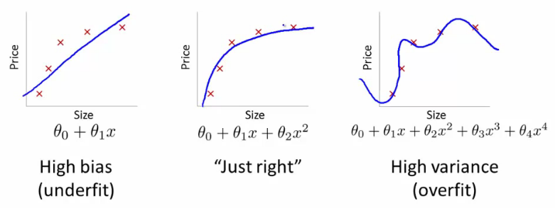
If we have too many features, the learned hypothesis may fit the training set very well:
But it may fail to generalize to new examples (let's say predict prices on new example of detecting if new messages are spam).
Here are couple of options that may be addressed:
- Reduce the number of features
- Manually select which features to keep
- Model selection algorithm
- Regularization
- Keep all the features, but reduce magnitude/values of model parameters (thetas).
- Works well when we have a lot of features, each of which contributes a bit to predicting y.
Regularization works by adding regularization parameter to the cost function:
In this case the gradient descent formula will look like the following:


