⭐ 2023-12-01: VerticaPy secures 200 stars.
📢 2020-06-27: Vertica-ML-Python has been renamed to VerticaPy.
📜 Some basic syntax can be found in the cheat sheet.
📰 Check out the latest newsletter here.
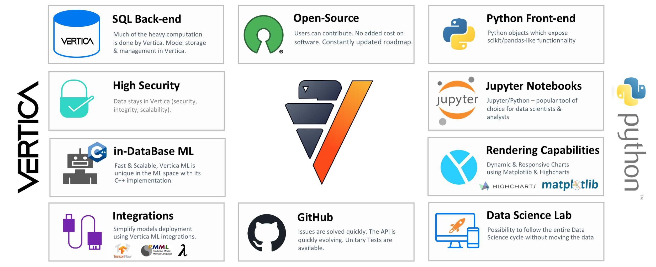
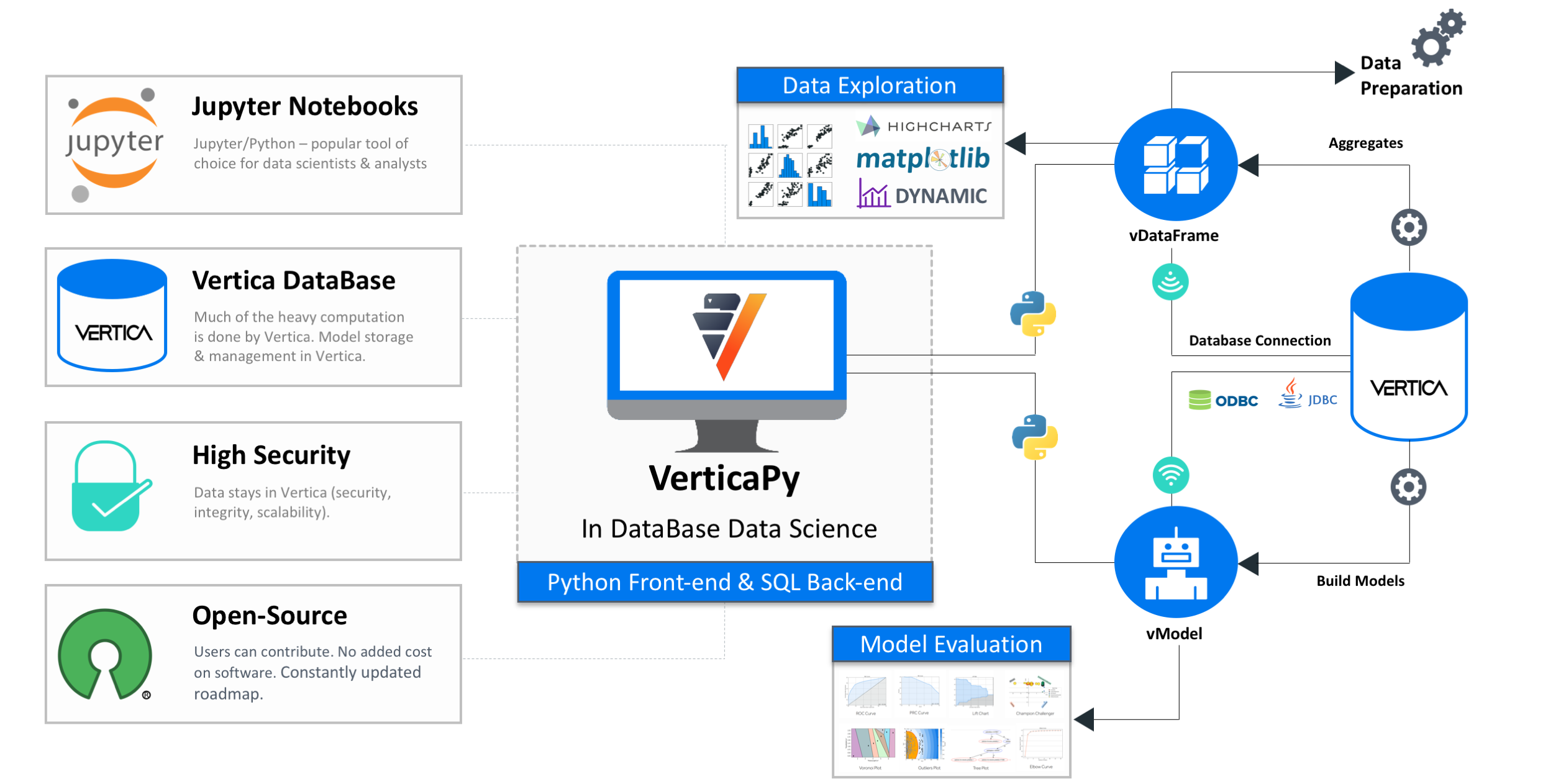
VerticaPy is a Python library with scikit-like functionality used to conduct data science projects on data stored in Vertica, taking advantage of Vertica’s speed and built-in analytics and machine learning features. VerticaPy offers robust support for the entire data science life cycle, uses a 'pipeline' mechanism to sequentialize data transformation operations, and offers beautiful graphical options.
- Introduction
- Installation
- Connecting to the Database
- Documentation
- Use-cases
- Highlighted Features
- Quickstart
- Help and Support
Vertica was the first real analytic columnar database and is still the fastest in the market. However, SQL alone isn't flexible enough to meet the needs of data scientists.
Python has quickly become the most popular tool in this domain, owing much of its flexibility to its high-level of abstraction and impressively large and ever-growing set of libraries. Its accessibility has led to the development of popular and perfomant APIs, like pandas and scikit-learn, and a dedicated community of data scientists. Unfortunately, Python only works in-memory as a single-node process. This problem has led to the rise of distributed programming languages, but they too, are limited as in-memory processes and, as such, will never be able to process all of your data in this era, and moving data for processing is prohobitively expensive. On top of all of this, data scientists must also find convenient ways to deploy their data and models. The whole process is time consuming.
VerticaPy aims to solve all of these problems. The idea is simple: instead of moving data around for processing, VerticaPy brings the logic to the data.
3+ years in the making, we're proud to bring you VerticaPy.
Main Advantages:
- Easy Data Exploration.
- Fast Data Preparation.
- In-Database Machine Learning.
- Easy Model Evaluation.
- Easy Model Deployment.
- Flexibility of using either Python or SQL.
To install VerticaPy with pip:
# Latest release version
root@ubuntu:~$ pip3 install verticapy[all]

# Latest commit on master branch
root@ubuntu:~$ pip3 install git+https://github.com/vertica/verticapy.git@master
To install VerticaPy from source, run the following command from the root directory:
root@ubuntu:~$ python3 setup.py installA detailed installation guide is available at:
https://www.vertica.com/python/documentation/installation.html
VerticaPy is compatible with several clients. For details, see the connection page.
The easiest and most accurate way to find documentation for a particular function is to use the help function:
import verticapy as vp

help(vp.vDataFrame)
Official documentation is available at:
https://www.vertica.com/python/documentation/
Examples and case-studies:
https://www.vertica.com/python/examples/
VerticaPy, offers users the flexibility to customize their coding experience with two visually appealing themes: Dark and Light.
Dark mode, ideal for night-time coding sessions, features a sleek and stylish dark color scheme, providing a comfortable and eye-friendly environment.
On the other hand, Light mode serves as the default theme, offering a clean and bright interface for users who prefer a traditional coding ambiance.
Theme can be easily switched by:
import verticapy as vp

vp.set_option("theme", "dark") # can be switched 'light'.
VerticaPy's theme-switching option ensures that users can tailor their experience to their preferences, making data exploration and analysis a more personalized and enjoyable journey.
You can use VerticaPy to execute SQL queries directly from a Jupyter notebook. For details, see SQL Magic:
Load the SQL extension.
%load_ext verticapy.sqlExecute your SQL queries.
%%sql
SELECT version();

# Output
# Vertica Analytic Database v11.0.1-0You can create interactive, professional plots directly from SQL.
To create plots, simply provide the type of plot along with the SQL command.
%load_ext verticapy.jupyter.extensions.chart_magic
%chart -k pie -c "SELECT pclass, AVG(age) AS av_avg FROM titanic GROUP BY 1;"In a single platform, multiple databases (e.g. PostgreSQL, Vertica, MySQL, In-memory) can be accessed using SQL and python.
%%sql
/* Fetch TAIL_NUMBER and CITY after Joining the flight_vertica table with airports table in MySQL database. */
SELECT flight_vertica.TAIL_NUMBER, airports.CITY AS Departing_City
FROM flight_vertica
INNER JOIN &&& airports &&&
ON flight_vertica.ORIGIN_AIRPORT = airports.IATA_CODE;
In the example above, the 'flight_vertica' table is stored in Vertica, whereas the 'airports' table is stored in MySQL. We can associate special symbols "&&&" to the different databases to fetch the data. The best part is that all the aggregation is pushed to the databases (i.e. it is not done in memory)!
For more details on how to setup DBLINK, please visit the github repo. To learn about using DBLINK in VerticaPy, check out the documentation page.
VerticaPy has a unique place in the market because it allows users to use Python and SQL in the same environment.
import verticapy as vp

selected_titanic = vp.vDataFrame(
    "(SELECT pclass, embarked, AVG(survived) FROM public.titanic GROUP BY 1, 2) x"
)
selected_titanic.groupby(columns=["pclass"], expr=["AVG(AVG)"])Verticapy comes integrated with three popular plotting libraries: matplotlib, highcharts, and plotly.
A gallery of VerticaPy-generated charts is available at:
https://www.vertica.com/python/documentation/chart.html
-
Data Ingestion
VerticaPy allows users to ingest data from a diverse range of sources, such as AVRO, Parquet, CSV, JSON etc. With a simple command "read_file", VerticaPy automatically infers the source type and the data type.
import verticapy as vp

read_file(
    "/home/laliga/2012.json",
    table_name="laliga",
)
As shown above, it has created a nested structure for the complex data. The actual file structure is below:
We can even see the SQL underneath every VerticaPy command by turning on the genSQL option:
  import verticapy as vp

  read_file("/home/laliga/2012.json", table_name="laliga", genSQL=True)
CREATE LOCAL TEMPORARY TABLE "laliga"
("away_score" INT,
"away_team" ROW("away_team_gender" VARCHAR,
"away_team_group" VARCHAR,
"away_team_id" INT, ...
ROW("id" INT,
"name" VARCHAR)),
"competition" ROW("competition_id" INT,
"competition_name" VARCHAR,
"country_name" VARCHAR),
"competition_stage" ROW("id" INT,
"name" VARCHAR),
"home_score" INT,
"home_team" ROW("country" ROW("id" INT,
"name" VARCHAR),
"home_team_gender" VARCHAR,
"home_team_group" VARCHAR,
"home_team_id" INT, ...),
"kick_off" TIME,
"last_updated" DATE,
"match_DATE" DATE,
"match_id" INT, ...
ROW("data_version" DATE,
"shot_fidelity_version" INT,
"xy_fidelity_version" INT),
"season" ROW("season_id" INT,
"season_name" VARCHAR))
ON COMMIT PRESERVE ROWS
COPY "v_temp_schema"."laliga"
FROM '/home/laliga/2012.json'
PARSER FJsonParser()VerticaPy provides functions for importing other specific file types, such as read_json and read_csv. Since these functions focus on a particular file type, they offer more options for tackling the data. For example, read_json has a "flatten_arrays" parameter that allows you to flatten nested JSON arrays.
-
Data Exploration
There are many options for descriptive and visual exploration.
from verticapy.datasets import load_iris

iris_data = load_iris()
iris_data.scatter(
    ["SepalWidthCm", "SepalLengthCm", "PetalLengthCm"],
    by="Species",
    max_nb_points=30
)
The Correlation Matrix is also very fast and convenient to compute. Users can choose from a wide variety of correaltions, including cramer, spearman, pearson etc.
from verticapy.datasets import load_titanic

titanic = load_titanic()
titanic.corr(method="spearman")
By turning on the SQL print option, users can see and copy SQL queries:
from verticapy import set_option

set_option("sql_on", True)
SELECT
/*+LABEL('vDataframe._aggregate_matrix')*/ CORR_MATRIX("pclass", "survived", "age", "sibsp", "parch", "fare", "body") OVER ()
FROM
(
SELECT
RANK() OVER (ORDER BY "pclass") AS "pclass",
RANK() OVER (ORDER BY "survived") AS "survived",
RANK() OVER (ORDER BY "age") AS "age",
RANK() OVER (ORDER BY "sibsp") AS "sibsp",
RANK() OVER (ORDER BY "parch") AS "parch",
RANK() OVER (ORDER BY "fare") AS "fare",
RANK() OVER (ORDER BY "body") AS "body"
FROM
"public"."titanic") spearman_tableVerticaPy allows users to calculate a focused correlation using the "focus" parameter:
titanic.corr(method="spearman", focus="survived")-
Data Preparation
Whether you are joining multiple tables, encoding, or filling missing values, VerticaPy has everything and more in one package.
import random
import verticapy as vp

data = vp.vDataFrame({"Heights": [random.randint(10, 60) for _ in range(40)] + [100]})
data.outliers_plot(columns="Heights")-
Machine Learning
ML is the strongest suite of VerticaPy as it capitalizes on the speed of in-database training and prediction by using SQL in the background to interact with the database. ML for VerticaPy covers a vast array of tools, including time series forecasting, clustering, and classification.
# titanic_vd is already loaded
# Logistic Regression model is already loaded
stepwise_result = stepwise(
    model,
    input_relation=titanic_vd,
    X=[
        "age",
        "fare",
        "parch",
        "pclass",
    ],
    y="survived",
    direction="backward",
    height=600,
    width=800,
)VerticaPy provides some predefined datasets that can be easily loaded. These datasets include the iris dataset, titanic dataset, amazon, and more.
There are two ways to access the provided datasets:
(1) Use the standard python method:
from verticapy.datasets import load_iris

iris_data = load_iris()
(2) Use the standard name of the dataset from the public schema:
iris_data = vp.vDataFrame(input_relation = "public.iris")The following example follows the VerticaPy quickstart guide.
Install the library using with pip.
root@ubuntu:~$ pip3 install verticapy[all]Create a new Vertica connection:
import verticapy as vp

vp.new_connection({
    "host": "10.211.55.14",
    "port": "5433",
    "database": "testdb",
    "password": "XxX",
    "user": "dbadmin"},
    name="Vertica_New_Connection")
Use the newly created connection:
vp.connect("Vertica_New_Connection")Create a VerticaPy schema for native VerticaPy models (that is, models available in VerticaPy, but not Vertica itself):
vp.create_verticapy_schema()Create a vDataFrame of your relation:
from verticapy import vDataFrame

vdf = vDataFrame("my_relation")
Load a sample dataset:
from verticapy.datasets import load_titanic

vdf = load_titanic()
Examine your data:
vdf.describe()Print the SQL query with set_option:
set_option("sql_on", True)
vdf.describe()

# Output
## Compute the descriptive statistics of all the numerical columns ##

SELECT
  SUMMARIZE_NUMCOL("pclass", "survived", "age", "sibsp", "parch", "fare", "body") OVER ()
FROM public.titanic
With VerticaPy, it is now possible to solve a ML problem with few lines of code.
from verticapy.machine_learning.model_selection.model_validation import cross_validate
from verticapy.machine_learning.vertica import RandomForestClassifier

# Data Preparation
vdf["sex"].label_encode()["boat"].fillna(method="0ifnull")["name"].str_extract(
    " ([A-Za-z]+)\."
).eval("family_size", expr="parch + sibsp + 1").drop(
    columns=["cabin", "body", "ticket", "home.dest"]
)[
    "fare"
].fill_outliers().fillna()

# Model Evaluation
cross_validate(
    RandomForestClassifier("rf_titanic", max_leaf_nodes=100, n_estimators=30),
    vdf,
    ["age", "family_size", "sex", "pclass", "fare", "boat"],
    "survived",
    cutoff=0.35,
)
# Features importance
model.fit(vdf, ["age", "family_size", "sex", "pclass", "fare", "boat"], "survived")
model.features_importance()# ROC Curve
model = RandomForestClassifier(
name = "public.RF_titanic",
n_estimators = 20,
max_features = "auto",
max_leaf_nodes = 32,
sample = 0.7,
max_depth = 3,
min_samples_leaf = 5,
min_info_gain = 0.0,
nbins = 32
)
model.fit(
"public.titanic", # input relation
["age", "fare", "sex"], # predictors
"survived" # response
)
# Roc Curve
model.roc_curve()Enjoy!
For a short guide on contribution standards, see the Contribution Guidelines.
-
Announcements and Discussion: https://github.com/vertica/VerticaPy/discussions


